Control Systems
— HimanishMathematical Models of Systems #
Laplace Transform #
| Time | Frequency |
|---|---|
| \(tf(t)\) | \(-F’(s)\) |
| \(t^nf(t)\) | \((-1)^nF^{(n)}(s)\) |
| \(f(t-a)u(t-a)\) | \(e^{-as}F(s)\) |
| \(f’(t)\) | \(sF(s)-f(0^-)\) |
| \(\frac{1}{t}f(t)\) | \(\int_s^{\infty}F(\sigma)d\sigma\) |
| \(e^{at}f(t)\) | \(F(s-a)\) |
| \(u(t-a)\) | \(e^{-as}/s\) |
| \(\delta(t)\) | 1 |
| \(t^n\) | \(\frac{n!}{s^{n+1}}\) |
| \(e^{-at}\) | \(\frac{1}{s+a}\) |
| \(\cos(\omega_0t) u(t)\) | \(\frac{s}{s^2+\omega_0^2}\) |
| \(\sin(\omega_0t) u(t)\) | \(\frac{\omega_0}{s^2+\omega_0^2}\) |
- The Laplace variable s can be considered as the differential operator, i.e.
\[s \equiv \frac{d}{dt}\] \[\frac{1}{s} = \int_{0^-}^tdt\]
- Used to solve differential equations, which arise when describing system behaviour.
- Coefficient A of partial fraction decomposition of \(Y(s)\), corresponding to pole \(p_1\) is given by
\[A = \lim_{s\to p_1}(s-p_1)Y(s)\]
Transfer Function #
\[G(s) = \frac{Y(s)}{R(s)}\]
Block Diagram #
Time Domain Analysis #
- DC Gain, \(K = G(s=0)\)
Response of a System #
- Time Response is for aperiodic inputs:
- Impulse
- Step
- Ramp
- Whereas frequency response is for periodic inputs (e.g. sinusoids)
| Input R(s) | |
|---|---|
| Impulse | 1 |
| Step | \(\frac{1}{s}\) |
| Ramp | \(\frac{1}{s^2}\) |
| Parabola (\(t^2/2\)) | \(\frac{1}{s^3}\) |
- To determine the steady state of response \(y(t)\), we may use the final value theorem: \[ y(t\to\infty) = \lim_{s\to0}sY(s)\]
Feedback Control System #
- A closed-loop system uses a measurement of the output signal and a comparison with the desired output to generate an error signal that is used by the controller to adjust the actuator.
- Error: \(E(s) = Y_{des}(s) - Y(s) = R(s) - Y(s)\)
- For a unity feedback system, \[E(s) = \frac{R(s)}{1+G(s)}\]
- So, steady state error: \[e_{ss}=\lim_{s \to 0} \frac{sR(s)}{1+G(s)}\]
First Order Systems #
\[G(s) = \frac{K}{\tau s + 1}\]
- Settling time = \(4\tau\)
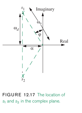
Second Order Systems #
\[G(s) = \frac{\omega_n^2}{s^2+2\xi\omega_ns+\omega_n^2}\]
Unit Step Response #
\[s_{1,2} = -\xi\omega_n\pm j\omega_d\] \(\omega_d = \omega_n\sqrt{1-\xi^2}\) \[\cos \theta = \xi, \ \sin\theta = \sqrt{1-\xi^2} \]
- Peak time \(t_p = \pi/\omega_d\) at which
- Peak overshoot: \(M_p = \exp(-\pi\xi/\sqrt{1-\xi^2})\cdot 100\%\)
- Rise time \[t_r = \frac{\pi-\theta}{\omega_d}\]
- Settling time
\[t_s = \begin{cases} \frac{3}{\xi\omega_n} & 5\% \text{ tolerance} \\ \frac{4}{\xi\omega_n} & 2\% \text{ tolerance} \end{cases} \]
Stability #
- A stable system is a dynamic system with a bounded response to a bounded input.
- Impulse response \(g(t)\) must be absolutely integrable.
- A necessary and sufficient condition for a feedback system to be stable is that all the poles of the system transfer function have negative real parts.
- A system is stable if all the poles of the transfer function are in the left- hand s-plane
- A system is not stable if not all the roots are in the left-hand plane.
- Marginally stable if simple roots on imaginary axis, with all other roots in left-hand plane.
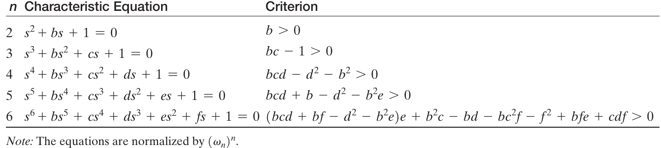
Routh Criterion #
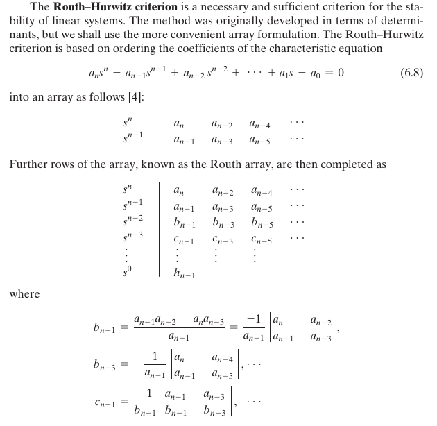
- For a stable system, there should be no changes in sign in the first column.
- The number of roots of the characteristic polynomial \(q(s)\) with positive real parts is equal to the number of sign changes in the first column of the array.
Root Locus #
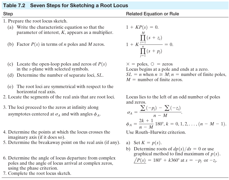
- Centroid and angles of asymptote have \((p-z)\) in the denominator
Angle of Departure #
\[\theta_d = 180^{\circ} - (\sum \theta_p - \sum \theta_z)\]
- \(\theta_p\) is the angle made by the pole/zero whose angle of departure is to be found w.r.t. other poles, i.e. angle made by a vector originating from other poles and ending at the pole in question with real axis.
- Angle of departure need not be calculated for poles/zeros on real axis as graph of root locus should be symmetric about real axis
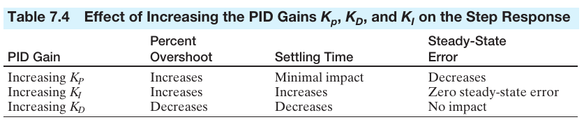
Controller Design #
- The control effort \(U(s)\) is the output given by the compensator i.e. \(U(s) = G_c(s)E(s)\)
- In general, a PID controller has a transfer function \[G_c(s) = K_p + \frac{K_I}{s}+ K_Ds\]
- When \(K_D = 0\), we have a proportional plus integral (PI) controller
- When \(K_I = 0\), we have a proportional plus derivative (PD) controller
- The PID controller can also be viewed as a cascade of the PI and the PD controllers.
- We cannot change settling time using a proportional compensator alone
- We can control \(\zeta\) or \(\omega_n\) but not both parameters
\[\cos\theta = \zeta \]
\[\alpha = \zeta\omega_n\]
Frequency Response #
Polar Plot #
- Put \(s = j \omega\)
- Find magnitude and phase of \(G(j\omega)\)
- Find points (mag, phase) at which \(\omega = 0\) and \(\omega = \infty\)
- Separate Real and Imaginary parts by multiplying with conjugate
- Points of intersection with Real axis and Imaginary axis
- Plot these four points (intersections with axes and 0 and \(\infty\)) and connect them
Gain Margin and Phase Crossover #
\[\omega_{pc} \ @ \ \operatorname{Im}{G(j\omega)} = 0 \] \[ GM = \frac{1}{|G(j\omega_{pc})|}\]
Phase Margin and Gain Crossover #
- Find \(\omega = \omega_{gc}\) for which
\[ |G(j\omega)| = 1\]
- Then \[PM = 180^{\circ} + \phi\] where \[\phi = \angle{G(j\omega_{gc})}\]
Stability in Frequency Domain #
Contours #
By convention, the area within a contour to the right of the traversal of the contour is considered to be the area enclosed by the contour. Therefore, we will assume clockwise traversal of a contour to be positive and the area enclosed within the contour to be on the right.
Nyquist Plot #
- Polar Plot
- Inverse Polar Plot
- Nyquist Contour
Nyquist Criterion #
- A transfer function is called a minimum phase transfer function if all its zeros lie in the left-hand s-plane. It is called a nonminimum phase transfer function if it has zeros in the right-hand s-plane.
- A feedback system is stable if and only if the contour in the L(s)-plane does not encircle the \((-1, 0)\) point when the number of poles in the right hand plane is zero.
- \(\omega_{pc} > \omega_{gc}\): stable system
- \(\omega_{pc} < \omega_{gc}\): unstable system
- \(\omega_{pc} = \omega_{gc}\): critically stable system
- If the number of poles in the RHP is not zero, the number of counterclockwise encirclements
- The \((-1, 0)\) point on Nyquist plot is same as the \(0 dB, -180^\circ\) point on Bode plot.
- The gain margin is the increase in the system gain when phase = −180° that will result in a marginally stable system with intersection of the \(−1 + j0\) point on the Nyquist plot.