electronics

Signals and Systems

Mon Jan 17, 2022 [Wed Nov 2, 2022]

Basics #

Signal: time-varying function that conveys information. Two types:
- Analog: can continuously take on any value in a range
- Digital: discretised. Fixed finite possible values.
Sample times can be discrete or continuous.
- Arrow indicates sample value is at n=0

Absolutely summable sequence: \[\sum_{-\infty}^{\infty} |x(n)| \le P < \infty\]
Square summable sequence: \[\sum_{-\infty}^{\infty} |x(n)|^2 \le Q < \infty\]

Energy #

Discrete #

\(E_{\infty} = \sum_{-\infty}^{\infty} |x[n]|^2\)

Continuous #

\[E_{\infty} = \int_{-\infty}^{\infty} |x(t)|^2dt\]

if \(x(t)\) and \(y(t)\) are orthogonal signals and \(z(t) = x(t) + y(t)\), then \[E_z = E_x + E_y\]

Power #

\[P = \lim_{T\to\infty} \frac{E}{T}\]

Power of

Discrete Time #

\[ P = \lim_{k \to\infty} \frac{1}{2k+1}\sum_{-k}^k|x(n)|^2 \]

Continuous Time #

\[ P = \lim_{T\to\infty} \frac{1}{2T}\int_{-T}^T|x(t)|^2 dt \]

Energy and Power Signals #

Energy Signal: Energy is finite, power is zero (\(P = \lim_{T\to\infty} \frac{E}{T}\))
Power Signal: Power is finite, energy is infinite
Neither Energy Nor Power Signal: Both are infinite

Every signal observed in real life is an energy signal. A power signal must have infinite duration.

Necessary Conditions #

Energy Signal

Must be
- Finite duration and Bounded
- Infinite duration, Bounded and Decaying

Power Signal
- Periodic signals are always power signals
Must be
- Bounded
- Infinite duration
- Not decaying

Transformations of Independent Variable #

\(x[n] \implies n \in \mathbb{Z}\) [discrete]
\(x(n) \implies\) continuous signal

Time Shrinkage #

Consider the function \(x(\alpha t)\):
- If \(\alpha > 1\): shrinks to \(\frac{1}{\alpha}\) of original (speed increases)
- If \(\alpha < 1\): expands to \(\alpha\) times original (slows down)
For discrete signal \(x[\alpha t]\):
- If \(\alpha > 1\): samples get skipped
- \(\alpha < 1\): Output for which input is fractional become zero

Time Shift #

\(x(t-t_0)\): Delayed if \(t_0 > 0\) else advanced
Example: \(x(-2t+6) = x(-2(t-3))\)
- First scale then shift: scaled by -2 and delayed by 3

Even and Odd Parts #

\[\mathcal{Ev}\{x(t)\} = \frac{x(t)+x(-t)}{2}\]
\[\mathcal{Od}\{x(t)\} = \frac{x(t)-x(-t)}{2}\]

Unit Impulse Signal #

CT #

Infinite at x=0, and zero otherwise
NENP signal

\(\frac{d}{dt}u(t) = \delta(t)\)

DT #

1 at n=0, and zero otherwise
Energy signal

Basic System Properties #

Memoryless System #

A system is memoryless if the output \(y(n)\) depends on the value of input \(x(n)\)at n only, for all values of n.

Invertible System #

Distinct inputs lead to distinct outputs.

Time-invariant System #

Delay at the input should produce an equal delay in output.

Rule of thumb: breaks if \(t\) outside \(x(t)\) or messing with \(t\) inside \(x(t)\) e.g. \(x(\frac{t}{3})\)

Causal System #

Output is independent of future values of input.

Noncausal System

Output depends on future inputs.

Anticausal System

Output depends purely on future values of input.

Stable System #

A stable system is one in which small inputs lead to responses that do not diverge.
Bounded inputs lead to bounded outputs.

Deterministic and Random Signals #

Deterministic signal: Physical description is known completely, either mathematical or graphical form
Random signal: Only known in terms of probabilistic description e.g. most noise signals

Approximating a Signal #

A signal \(g(t)\) is approximated by another signal \(x(t)\) as \[g(t) \approx cx(t)\] when \[ c = \frac{\int_{t_1}^{t_2} g(t)x(t)dt}{\int_{t_1}^{t_2}x^2(t)dt} = \frac{1}{E_x} \int_{t_1}^{t_2}g(t)x^{*}(t)dt\]

Correlation #

Similiarity index \[\rho := \frac{1}{\sqrt{E_gE_x}}\int_{-\infty}^{\infty}g(t)x^{*}(t)dt\]

Cross-correlation #

\[\psi_{zg}(\tau) := \int_{-\infty}^{\infty}z(t)g^{*}(t-\tau)dt\]

Autocorrelation #

\[\psi_g(\tau) := \int_{-\infty}^{\infty}g(t)g(t+\tau)dt\]

Linear Time-Invariant Systems #

DT LTI Systems #

DT Signals as Impulse Sums #

\[x[n] = \sum_{k=-\infty}^{\infty}x[k]\delta[n-k]\]
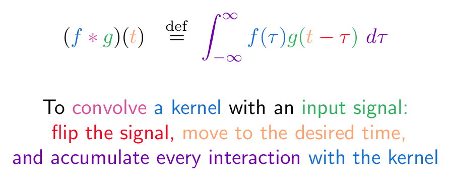
Convolution sum

\[y[n] = x[n] * h[n] ::= \sum_{k=-\infty}^{\infty}x[k]h[n-k]\]

\(h[n]\) is the output of the system when \(\delta[n]\) is the input

Properties of LTI Systems #

Commutativity #

\[x[n] * h[n] = h[n] * x[n]\]

Distributivity #

\[x * (h_1 + h_2) = x * h_1 + x * h_2\]

Associativity #

\[x * (h_1 * h_2) = (x * h_1) * h_2\]

Memory #

If the output at some time should depend only on the input’s value at that time, then \(h[n] = 0 \text{ if } n \ne 0\)
\[h[n] = K \delta [n]\]

\(K = h[0]\)

Thus \(y[n] = Kx[n]\)

Invertibility #

If the inverse system has impulse response \(h_1(t)\) then \[h(t) * h_1(t) = \delta(t)\]

Causality #

For a causal system, \[h(t) = 0 \text{ for } t < 0\]

Stability #

The impulse response must be absolutely integrable for \(y(t)\) to be bounded, and the system to be stable, i.e. \[\int_{-\infty}^{\infty} |h(\tau)|d\tau < \infty\]

Unit Step Response #

The unit step response \(s[n]\) of a system corresponds to the output when \(x[n] = u[n]\) \[s[n] = u[n] * h[n]\]

\[s[n] = \sum_{\infty}^n h[k]\]
- \[h[n] = s[n] - s[n-1]\]

System Description Via Diff Equations #

Fourier Series #

\[x(t) = \sum_{-\infty}^{\infty}a_ke^{jk\omega_0t}\] Continuous: \[ a_k = \frac{1}{T} \int_T x(t)e^{-jk\omega_0t}dt \] Discrete:\[ a_k = \frac{1}{N} \sum_N x[n]e^{-jk\omega_0n} \]

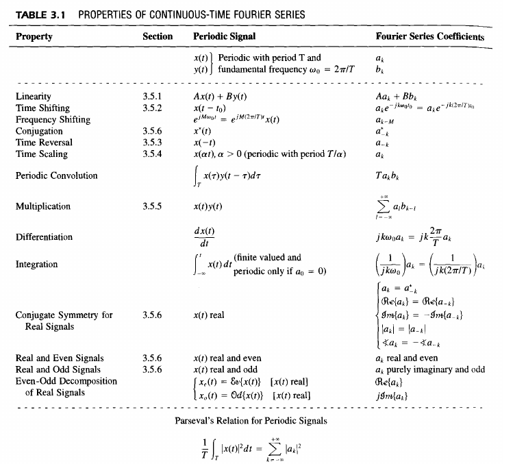
For a signal to be real valued, \(a_k^* = a_{-k}\)
For a signal to be even, \(a_k\) should be even.

Frequency Response (LTI Systems) #

\[H(j\omega) = \sum_{n=-\infty}^{\infty}h[n]e^{-j\omega n}\] \[H(j\omega) = \int_{=-\infty}^{\infty}h(t)e^{-j\omega t}dt\] \[x(t) = \sum_{k=-\infty}^{\infty}a_ke^{jk\omega_0 t}\] \[y(t) = \sum_{k=-\infty}^{\infty}a_kH(jk\omega_0)e^{jk\omega_0t}\]

Fourier Transform #

\[x(t) = \frac{1}{2\pi}\int_{-\infty}^{\infty}X(j\omega)e^{j\omega t}d\omega\] \[X(j\omega) = \int_{-\infty}^{\infty}x(t)e^{-j\omega t}dt\]

Periodic Signals #

\[X(j\omega) = \sum_{k=-\infty}^{\infty}2\pi a_k\delta(\omega-k\omega_0)\]

Filters #

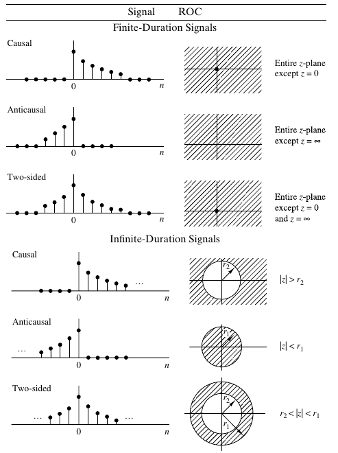
Z-Transform #

Absolutely summable signal: ROC must include unit circle
Finite length signal: ROC must include entire z-plane