Deep Learning

Wed Jan 26, 2022 [Sun Apr 9, 2023]

Neural Networks #

Several binary inputs, single binary output
Device that makes decisions by weighing up evidence
Output is 1 if \(w \cdot x = \sum_jw_jx_j\) crosses a threshold, else 0
A many-layer network of perceptrons can engage in sophisticated decision making: the second layer makes decisions at a more abstract and complex level than the first.
We use a bias term \(b\) which measures how easy it is to get the perceptron to fire. A really big bias, easy to output a 1. So:

\[ \text{output} = \begin{cases} 0 & w \cdot x + b \le 0 \\ 1 & w \cdot x + b > 0 \end{cases} \]

A perceptron can be used as a NAND gate. So a network can be used to compute any logical function.

We want the network to learn weights and biases. Suppose we make a small change in some weight (or bias) in the network. What we’d like is for this small change in weight to cause only a small corresponding change in the output from the network
But, a small change in the weights or bias of any single perceptron in the network can sometimes cause the output of that perceptron to completely flip
So we need a new type of artificial neuron called a sigmoid neuron, which is just like a perceptron but the output is \(\sigma(w \cdot x + b)\) where the sigmoid function is defined by \[\sigma(z) = \frac{1}{1+e^{-z}}\]
This is a smoothed version of a step function, which means small changes in weights and bias will produce a small change in the output.

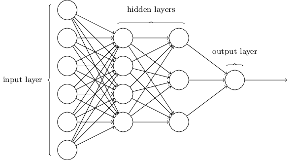
Feedforward NNs: information is always fed forward, never fed back
Recurrent neural networks: feedback loops are possible. Neurons which fire for some limited duration of time, before becoming quiescent. That firing can stimulate other neurons.
- Less influential as their algos are less powerful for the time being, but these networks are closer to how our brain works.

4 neurons are enough to represent \(2^4\) values
Let’s concentrate on the first output neuron, the one that’s trying to decide whether or not the digit is a 0. It does this by weighing up evidence from the hidden layer of neurons
If we had 4 outputs, then the first output neuron would be trying to decide what the most significant bit of the digit was. It’s hard to imagine that there’s any good historical reason the component shapes of the digit will be closely related to (say) the most significant bit in the output.

To quantify how well our algorithm is achieving finding the weights and biases, we define a cost function (or loss/objective function)

\[ C(w,b) \equiv \frac{1}{2n} \sum_x \| y(x) - a\|^2 \]

\(a\): vector of outputs when x is input
\(C\): mean squared error (MSE)
The cost becomes small, i.e., \(C(w,b)≈0\), precisely when y(x) is approximately equal to the output, a, for all training inputs, x. And vice-versa.
We need to minimise the cost, which we’ll do using gradient descent.
We can’t maximise the number of images classified correctly, because that is not a smooth function of weights and biases, which makes it difficult to figure how to change them. Whereas small changes can be easily made to weights and biases if we use quadratic cost.

\[ \Delta C \approx \nabla C \cdot \Delta v\] where \[\nabla C \equiv \left(\frac{\partial C}{\partial v_1}, \ldots, \frac{\partial C}{\partial v_m}\right)^T\]
Choose \(\Delta v = -\eta \nabla C\) so the update rule for gradient descent becomes \[v \rightarrow v’ = v-\eta \nabla C\]
Apply the constraint that \(\| \Delta v \| = \epsilon\). It can be proved using the Cauchy-Schwarz inequality that \(\eta = \epsilon / \|\nabla C\|\) minimises \(\nabla C \cdot \Delta v\)
To roll down the hill, apply \[w_k \rightarrow w_k’ = w_k-\eta \frac{\partial C}{\partial w_k} \\ b_l \rightarrow b_l’ = b_l-\eta \frac{\partial C}{\partial b_l}\]

To speed up learning, since computing the gradients for all training inputs can take time, we use stochastic gradient descent
The idea is to estimate the gradient \(∇C\) by computing \(∇C_x\) for a small sample of randomly chosen training inputs
By averaging over this small sample it turns out that we can quickly get a good estimate of the true gradient
Stochastic gradient descent works by randomly picking out a small number m of randomly chosen training inputs. We’ll label those random training inputs \(X_1,X_2,…,X_m\), and refer to them as a mini-batch. Provided the sample size \(m\) is large enough we expect that the average value of the \(∇C_{X_j}\) will be roughly equal to the average over all \(∇C_x\), that is,

\[ \nabla C \approx \frac{1}{m} \sum_{j=1}^m \nabla C_{X_{j}} \]

Activation of the \(j^{th}\) neuron in the \(l^{th}\) layer is related to the activations in the \((l-1)^{th}\) layer

\[ a^{l}_j = \sigma\left( \sum_k w^{l}_{jk} a^{l-1}_k + b^l_j \right) \]

Taking the components of \(\sigma(v)\) as \(\sigma(v)_j = \sigma(v_j)\),\[ a^{l} = \sigma(w^l a^{l-1}+b^l)\]
- We just apply the weight matrix to the activations, then add the bias vector, and finally apply the \(\sigma\) function
- The intermediate quantity \(z^l \equiv w^l a^{l-1}+b^l \) is called the weighted input to neurons in layer \(l\)

Suppose s and t are vectors of the same dimension. Then the Hadamard product is the elementwise product of the two vectors.
The components of \(s \odot t\) are \[(s \odot t)_j = s_j t_j\]