Algorithms

“Perhaps the most important principle for the good algorithm designer is to refuse to be content.”

― Alfred V. Aho

Basics #

• Always ask yourself, “CAN WE DO BETTER?”
• Try to translate all pseudocode into code in some language

Guiding Principles #

1. We do a worst case analysis, appropriate for ‘general-purpose’ routines. As opposed to ‘average-case’ analysis, which requires domain knowledge

2. We don’t really pay much attention to constant factors, and lower order terms. Constant factors depend on the code implementation, architecture etc anyway. Not much predictive power is lost too, and makes our job easier.

   • Programming libraries do take into account constant factors for deciding when to switch from a particular algorithm to another

3. Asymptotic analysis: Focus on running time for large input sizes n. For small inputs, we don’t really need algorithm ingenuity

Asymptotic Analysis #

Big Oh #

\[T(n) = \mathcal{O}(f(n)) \implies \exists \ c, n_0 \text{ such that } T(n) \le cf(n) \ \ \forall n \ge n_0\]

Omega #

\[T(n) = \Omega(f(n)) \implies \exists \ c, n_0 \text{ such that } T(n) \ge cf(n) \ \ \forall n \ge n_0\]

Theta #

\[T(n) = \theta(f(n)) \text{ iff } T(n) = \mathcal{O}(f(n)) \text{ and } T(n) = \Omega(f(n)) \]

Little Oh #

\[T(n) = o(f(n)) \text{ iff } \forall \ c>0 \ \exists \ n_0 \text{ such that } T(n) \le cf(n) \ \forall \ n \ge n_0\]

Recursive Algorithms #

Generating Subsets #

void search(int k) {
  if (k == n+1) {
    // process subset
  } else {
    // include k in the subset
    subset.push_back(k);
    search(k+1);
    subset.pop_back();

    // don’t include k in the subset
    search(k+1);
}

• The function maintains a vector<int> subset that contains the element of each subset
• When the function search is called with parameter k, it decides whether to include the element k in the subset or not, and in both cases, then calls itself with parameter k+1. Then, if k = n+1, the function notices that all elements have been processed and a subset has been generated.

Divide and Conquer Paradigm #

Karatsuba Multiplication #

• Input: 2 n-digit numbers x, y
• Output: x*y
• Grade school algorithm: \(\mathcal{O}(n^2)\)
• Karatsuba: recursive, write \(x = 10^{n/2}a+b\) and \(y = 10^{n/2}c+d\)
• Then, \(xy = 10^nac+10^{n/2}(ad+bc)+bd\). Thus, halved the length of numbers being multiplied. Now recursively calculate the products ac, ad, bc, bd with the base case being primitive multiplication. Or even better, use Gauss’ trick to reduce recursive calls to 3 by calculating ad+bc directly:
  • \(ad+bc = (a+b)(c+d) - ac - bd\)
• Finally, pad zeros as per the powers of ten and use regular addition.

Merge Sort #

Merging two halves #

• First recursively sort first half of array and then recursively sort second half, then merge them using the following pseudocode

C: output array[n]
A: 1st sorted array[n/2]
B: 2nd sorted array[n/2]
for k = 1 to n
    if A(i) < B(j)
        C(k) = A(i)
        i++
    else
        C(k) = B(j)
        j++
end

Running Time #

• Running Time of Merge \(\leq 4m+2 \leq 6m\)
• Therefore, running time of merge sort is \(\leq 6n (\log n + 1)\)
• \(\log n\) is the number of times you divide n by 2 to get to 1
• Proof: using recursion tree method, a way to count work done by algo.

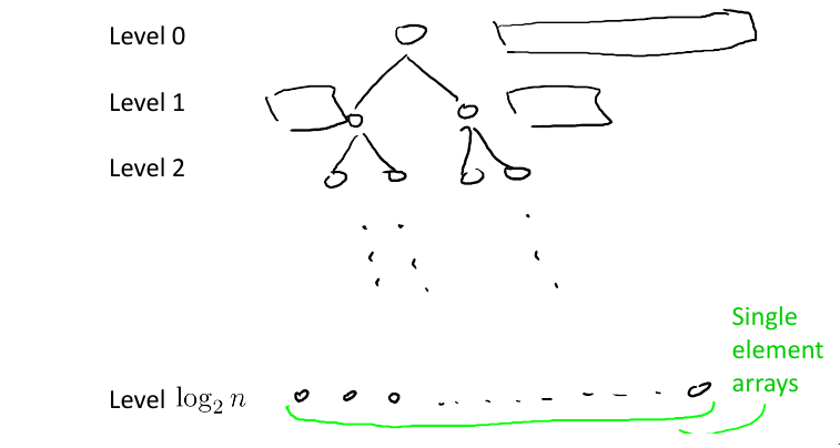
• At each level \(j = 0..\log n\), there are \(2^j\) subproblems, each of size \(n/2^j\)
• Therefore total operations at level j \(\leq 2^j * 6(n/2^j) = 6n\)
• Total work done by algo = Work per level * Number of levels = \(6n (\log n + 1)\)

Counting Array Inversions #

Problem #

• Input: Array with integers 1, 2, … in some arbitary order
• Output: Number of inversions i.e. number of pairs of array indices with i < j but A[i] > A[j]
• Motivation: measuring similarity between two ranked lists, relevant for making good recommendations to someone based on your knowledge of their and others’ preferences (“collaborative filtering”).
• Brute-force would cost \( \mathcal{O}(n^2)\)

Divide (into smaller subproblems) #

Differentiate between inversions and count them separately:

• Left inversion: if \(i, j \le n/2\)
• Right inversion: if i, j > n/2
• Split inversion: if i < n/2 < j

So now we need an algorithm somewhat like:

Count (array A, length n):
if n = 1 return 0
else
    x = Count(1st half of A, n/2)
    y = Count(2nd half of A, n/2)
    z = CountSplitInv(A, n)  ; to be implemented
    return x+y+z

We want CountSplitInv to be linear (\(\mathcal{O}(n)\)) so that Count will run in \(\mathcal{O}(n\log n)\). (just like merge sort)

Conquer (via recursive calls) #

Idea: Have recursive calls both count, and sort.

• Motivation? Merge sort’s merge subroutine naturally uncovers split inversions.
• How? If two sorted sub-arrays B and C each of size n/2 have no split inversions, then every element in B would be smaller than C, so the merge subroutine applied to these two would just concatenate them.
• So, every time an element from C is copied before B, it is a deviation from the trivial case, which means there are split inversions.
  • But how many? Every element left to copy from B at the time the element Y from C is copied would form a split inversion pair with Y.

Strassen’s Subcubic Matrix Multiplication #

• Very non-trivial algorithm
• Input size: \(\mathcal{O}(n^2)\), so the best an algorithm could do is \(\mathcal{O}(n^2)\)
• Trivial algorithm would be \(\mathcal{O}(n^3)\)

Divide #

• Divide the matrix into quadrants, similiar to how we divided a number into halves in Karatsuba multiplication.
• The quadrants behave like normal matrix elements for matrix multiplication i.e. if

\[ X =\left(\begin{array}{c|c} A & B \\ \hline C & D \end{array}\right), \quad Y =\left(\begin{array}{c|c} E & F \\ \hline G & H \end{array} \right) \] then\[ X =\left(\begin{array}{c|c} AE+BG & AF+BH \\ \hline CE+DG & CF+DH \end{array} \right) \]

Trivial Recursive Algorithm #

1. Recursively calculate the eight subproducts
2. Do the necessary additions (\(\mathcal{O}(n^2)\))

Sadly, this algorithm cannot beat \(\mathcal{O}(n^3)\) time.

Strassen’s Approach #

1. Recursively calculate only 7 products
2. Do the necessary (clever) additions and subtractions

The reduction of recursive calls from 8 to 7 changes the algorithm from cubic to subcubic time.

Master Method #

• Black box for solving recurrences
• Assumption: All subproblems have equal size

Recurrence Format #

T(n): maximum number of operations done by algorithm

1. Base Case: \(T(n) \le \text{a constant} \) for sufficiently small n

2. For larger n: \[T(n) \le aT(n/b)+\mathcal{O}(n^d)\]

   • a: number of recursive calls (\(\ge 1\))

   • b: factor by which input size shrinks (\(\ge 1\))

   • d: exponent in running time of combine step (work done outside recursive calls) (\(\ge 0\))

Master Theorem #

\[T(n) = \begin{cases} \mathcal{O}(n^d \log n) & a = b^d \\ \mathcal{O}(n^d) & a < b^d \\ \mathcal{O}(n^{\log_ba}) & a > b^d \end{cases}\]

• Interpretation:
  • a: Rate of subproblem proliferation
  • \(b^d\): rate of work shrinkage (per subproblem)

Randomised Algorithms #

QuickSort #

• Works in place, i.e. minimal extra memory needed unlike MergeSort

Partitioning around a Pivot #

1. Pick element of array (the “pivot”)
2. Rearrange array so that
   1. Left of pivot \(\rightarrow\) less than pivot
   2. Right of pivot \(\rightarrow\) greater than pivot

This takes \(\mathcal{O}(n)\) time with no extra memory involved. And it reduces the problem size, i.e. divide-n-conquer approach.

High-level description #

QuickSort(array A, length n)
    if n=1: return
    p = ChoosePivot(A, n)
    Partition A around p
    QuickSort(1st part)
    QuickSort(2nd part)

Pseudocode for Partition #

Let input: \(A[\ell \cdots r]\)

Partition (A, l, r)
    p := A[l]
    i := l+1
    for j = l+1 to r
        if A[j] < p  ; if A[j] > p, do nothing
            swap A[j], A[i]
            i := i+1
    swap A[l], A[i-1] ; bring pivot in between

Choosing a Pivot #

• Best case: Already sorted array, pick the median element, as we want the two subproblems to be of equal size as much as possible. Otherwise
• Choose the pivot randomly!
• Intuition: A 25-75 split is good enough for \(\mathcal{O}(n \log n)\) running time.
• If we have 100 numbers in an array, any number between 26 and 75 inclusive will give a 25-75 split or better. This has 50% probability, so we don’t need to be all that lucky for a good split
• QuickSort Theorem: For every array of length n, average running time of QuickSort (with random pivots) is \(\mathcal{O}(n \log n)\). Worst case, \(\mathcal{O}(n^2)\)

Time Complexity Analysis #

• Notations:
  • Sample space: \(\Omega\)
  • Random choices: \(\sigma\)
  • \(z_i = i^{th} \text{smallest element of array A i.e.} i^{th} \text{ order statistic} \)
• Key random variable:

\(C(\sigma) = \text{\# of comparisons between two elements made by QSort} \), as running time of QSort is dominated by comparisons.

• We can’t apply the Master Method as the subproblems are random, unbalanced.
• For indices \(i < j\), let \(X_{ij} = \text{\# of times } z_i, z_j \text{ get compared} \).
  • Now the only comparisons that occur are between the pivot and \(z_i\). Once an element has been compared with the pivot, the pivot would be excluded from further recursive calls, hence they would never be compared again.
• So, \(C(\sigma) = \sum_{i=1}^{n-1}\sum_{j=i+1}^n X_{ij}(\sigma)\)
  • \(E[C] = \sum_{i=1}^{n-1}\sum_{j=i+1}^n E[X_{ij}]\)
  • \(E[X_{ij}] = 0\cdot P[X_{ij}=0] + 1\cdot P[X_{ij}=1] = P[X_{ij}=1]\)
• \(P[z_i,z_j \text{ get compared}] = \frac{2}{j-i+1}\)
• \(E[C] = 2\sum_{i=1}^{n-1}\sum_{j=i+1}^n \frac{1}{j-i+1}\)
• Hence, \(E[C] \le 2 \cdot n \cdot \sum_{k=2}^n \frac{1}{k} \le 2n\ln n\)

Linear-Time Selection #

Input: Array A with n distinct numbers and a number \(i \in \{1…n\}\) Output: \(i^{th}\) order statistic i.e. \(z_i\) Example: \(i = (n+1)/2 \text{ for n odd}, i = n/2 \text{ for n even} \)

Trivial algorithm #

\(\mathcal{O}(n\log n)\)

1. Apply MergeSort
2. Return \(i^{th}\) element of sorted array

Randomised Selection #

RSelect (array A, length n, order statistic i)
    if n=1: return A[1]
    choose pivot P from A at random
    partition A around p, let j: new index of p
    if j=i: return p
    if j>i: return RSelect(1st part of A, j-1, i)
    if j<i: return RSelect(2nd part of A, n-j, i-j)

Graphs #

Ingredients #

• Vertices aka nodes (V: set of vertices)
  • \(n\): number of vertices
• Edges (E) aka arcs: pairs of vertices
  • undirected: unordered pair
  • directed: ordered pair
• \(m\): number of edges

Cuts #

• A cut of a graph (V, E) is a partition of V into two non-empty sets A and B.
• Possible cuts of a graph with n vertices = \(2^n-2\)
• Crossing edges: of a cut (A, B) are those with:
  • one endpoint in each of (A, B) [undirected]
  • tail in A, head in B [directed]

Minimum Cut Problem #

• Input: An undirected graph G = (V, E)
• Output: Compute a cut with fewest number of crossing edges

Karger’s Algorithm #

• While there are more than 2 vertices:
  • Pick a remaining edge \((u, v)\) uniformly at random
  • Merge (“contract”) u and v into a single vertex
  • Remove self-loops
• Return cut represented by final 2 vertices (i.e. all nodes in one supernode go to A and other supernode to B)

• Probability of success

Representation #

Sparse vs Dense #

In most applications, m (number of edges) is \(\Omega(n)\) and \(\mathcal{O}(n^2)\)

• In a sparse graph, m is \(\mathcal{O}(n)\) or close
• In a dense graph, m is closer to \(\mathcal{O}(n^2)\)

Adjacency Matrix #

• Represent G by a \(n \times n\) matrix A, where \(A_{ij} = 1 \Leftrightarrow G \text{ has an } i-j \text{ edge}\)
• Requires \(\theta(n^2)\) space
• useful for dense, gets wasteful for sparse graphs

Variants

• If parallel edges, \(A_{ij} = \) # of i-j edges
• \(A_{ij} = \) weight of i-j edge (if any)

Adjacency List #

• Ingredients
  • Array of vertices, \(\theta(n)\)
  • Array of edges, \(\theta(m)\)
  • Each edge points to its endpoints, \(\theta(m)\)
  • Each vertex points to edges incident on it, \(\theta(m)\)
• Requires \(\theta(m + n)\) storage space
• Better for sparse graphs
• Perfect for graph search algorithms

Traversal #

BFS #

marked = [False] * G.size()
def bfs(G, v):
    queue = [v]
    while len(queue) > 0:
        v = queue.pop(0)
    if not marked[v]:
        visit(v)
        marked[v] = True
        for w in G.neighbours(v):
            if not marked[w]:
                queue.append(w)

DFS #

• Recursive

Cleaner and easier to read

marked = [False] * G.size()
def dfs(G, v):
    visit(v)
    marked[v] = True
    for w in G.neighbours(v):
        if not marked[w]:
            dfs(G, w)

• Iterative

More generalisable

marked = [False] * G.size()
def dfs_iter(G, v):
    stack = [v]
    while len(stack) > 0:
        v = stack.pop()
        if not marked[v]:
            visit(v)
            marked[v] = True
            for w in G.neighbours(v):
                if not marked[w]:
                    stack.append(w)

Data Structures #

• Choose the minimal data structure that supports all the operations you need.

Sets and Multisets #

Policy-Based Sets #

Maps #

Queues and Dequeues #

Trees #

Binary Search Tree #

A binary search tree is a binary tree where for every node, any descendant of Node.left has a value strictly less than Node.val, and any descendant of Node.right has a value strictly greater than Node.val.

DFS #

• Three popular tree traversal orderings:
  • pre-order: first process the root node, then traverse the left subtree, then traverse the right subtree
  • in-order: first traverse the left subtree, then process the root node, then traverse the right subtree
  • post-order: first traverse the left subtree, then traverse the right subtree, then process the root node
• If we know the pre-order and in-order of a tree, we can reconstruct its exact structure. Same with post-order and in-order. But not post and pre.

BFS #

1) Create an empty queue q
2) temp_node = root (start from root)
3) Loop while temp_node is not NULL
    a) print temp_node->data.
    b) Enqueue temp_node’s children
      (first left then right children) to q
    c) Dequeue a node from q.

void printLevelOrder(TreeNode* root) {
// Base Case
  if (!root) return;
// Create an empty queue for level order traversal
  queue<TreeNode*> q;

// Enqueue Root and initialize height
  q.push(root);
  while (q.empty() == false) {
// Print front of queue and remove it from
    queue TreeNode* node = q.front();
    cout << node->data << " "; q.pop();

// Enqueue left child
    if (node->left) q.push(node->left);

// Enqueue right child
    if (node->right) q.push(node->right);
  }
}

Heaps #

Container for objects that have keys

• Canonical use of heap: Fast way to do repeated minimum calculations
  • HeapSort (SelectionSort with a heap [\(\mathcal{O}(n \log n)\)])
  • Event Manager [priority queue]
  • Median Maintanence

Supported Operations #

Both operations: \(\mathcal{O}(\log n)\)

• Insert: Add a new object to heap
  • Mass Insert would take \(\mathcal{O}(n \log n)\), better to use Heapify, which takes \(\mathcal{O}(n)\) for n batched Inserts
• Extract-Min: Remove an object in heap with min key value. (Supports Extract-Max equally well, but not both at the same time)
  • Mass removal can be done by Delete in \(\mathcal{O}(\log n)\)

Priority Queue #

• Multiset that supports
  • Insert: \(\mathcal{O}(\log n)\)
  • Extract-Min/Extract-Max (but not both together): retrieval and removal in \(\mathcal{O}(\log n)\)
  • Only retrieval: \(\mathcal{O}(1)\)
• Based on a heap

C++ #

priority_queue<int> max; // based on Max-Heap
max.push(3);
cout << max.top() << '\n';
max.pop();
priority_queue<int,vector<int>,greater<int>> min; // Min-Heap

Balanced BST #

• A sorted array but with fast (logarithmic) inserts+deletes

Supported Operations #

• \(\mathcal{O}(\log n)\): Search, Select (\(z_i\)), Min/Max, Pred/Succ, Rank, Insert, Delete
• \(\mathcal{O}(n)\): Output in Sorted Order

Comparison with Heap and Hash Table #

• Prefer heap when you only need: (as constant factors are smaller)
  • Insert
  • Delete
  • Min
• Prefer hash table (constant time look ups) when you don’t need min/max, and ordering on keys, i.e. only need to know what’s there and what’s not.

Greedy Algorithms #

• Iteratively make myopic decisions, and hope everything works out in the end.
• DANGER: Most greedy algorithms are NOT correct

Contrast with Divide and Conquer #

• Easy to propose (vs eureka moments)
• Easy running time analysis (vs Master Method etc)
• Hard to establish correctness (vs straightforward induction)

Scheduling #

• Shared resource e.g. processor working on many jobs (processes)
• What order should they be sequenced in, if each job has a:
  • Weight \(w_j\) (priority)
  • Length \(l_j\)
• Task: Minimise the weighted sum of completion times i.e. \(\text{min}\sum_{j=1}^nw_jC_j\) where
  • \(C_j\): sum of job lengths up to and including j.

Intuition #

• With equal lengths, we would schedule larger jobs earlier and with equal weights, schedule shorter jobs earlier.

Conflict Resolution #

What if \(w_i > w_j\) but also \(l_i > l_j\)?

• So, assign a ‘score’ to jobs which:
  • increases with weight
  • decreases with length
• Possible metrics:
  1. \(w_j-l_j\)
  2. \(w_j/l_j\)

Which One? #

Find an example where two algorithms produce different outputs, at least one has to be wrong! So, \(l_1 = 5, w_1 = 3\) [bigger diff] \(l_2 = 2, w_2 = 1\) [larger ratio]

On comparing weighted sums, we see that Alg #1 gives the wrong answer. So we use Alg #2 [proof of correctness by exchange argument], which has running time \(\mathcal{O}(n \log n)\) [sorting].

Huffman Codes #

• Binary code: Maps each character of an alphabet \(\Sigma\) to a binary string.
• Variable-length codes can lead to shorter encodings with non-uniform character frequencies by using lesser bits for the more frequent characters.
• To avoid ambiguity, we need prefix-free codes: for every pair \(i, j \in \Sigma\), neither of the encodings \(f (i), f (j)\) is a prefix of the other, e.g. {0,10,110,111}

Codes as Trees #

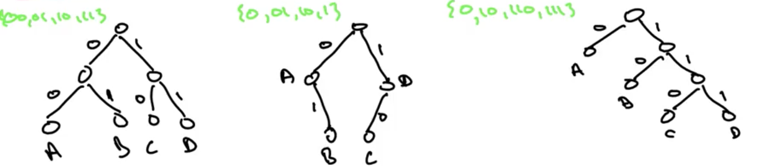
• We see that for prefix-free coding, only leaves should be labelled

Problem Statement #

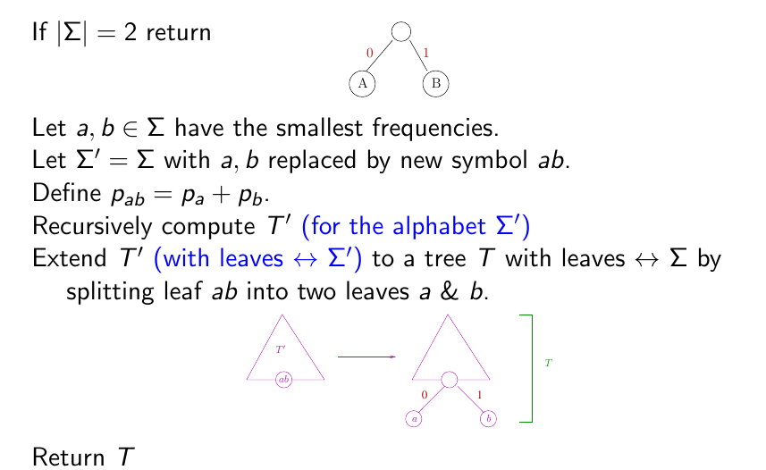
• Input: Probability \(p_i\) for each character \(i \in \Sigma\)
• If \(T\): tree with leaves \(\leftrightarrow\) symbols of \(\Sigma\), then \(L(T) = \sum\limits_{i \in \Sigma}p_i\cdot [\text{depth of i in T}] \)
• Output: Binary tree \(T\) minimising the average encoding length \(L(T)\)

Huffman’s Algorithm #

Amortised Analysis #

Two Pointers Method #

Two pointers walk through an array.

• Both pointers move to one direction only.

Sliding Window #

Shrinkable Window #

int i = 0, j = 0, ans = 0;
for (; j < N; ++j) {
    // CODE: use A[j] to update state which might make the window invalid
    for (; invalid(); ++i) { // when invalid, keep shrinking the left edge until it's valid again
        // CODE: update state using A[i]
    }
    ans = max(ans, j - i + 1); // the window [i, j] is the maximum window we've found thus far
}
return ans;

Non-Shrinkable Window #

int i = 0, j = 0;
for (; j < N; ++j) {
    // CODE: use A[j] to update state which might make the window invalid
    if (invalid()) { // Increment the left edge ONLY when the window is invalid. In this way, the window GROWs when it's valid, and SHIFTs when it's invalid
        // CODE: update state using A[i]
        ++i;
    }
    // after `++j` in the for loop, this window `[i, j)` of length `j - i` MIGHT be valid.
}
return j - i; // There must be a maximum window of size `j - i`.

Dynamic Programming #

#justdoit

Union Find (Disjoint Set) #

• Keep track of elements split into disjoint sets.

Applications #

• Kruskal’s MST Algorithm
• LCA in Trees
• Grid percolation

Time Complexities #

• Construction: \(\mathcal{O}(n)\)
• Union: \(\alpha(n)\) [\(\alpha\): amortised constant time]
• Find: \(\alpha(n)\)
• Count components: \(\mathcal{O}(1)\)

Kruskal’s MST #

Minimum Spanning Tree (may not be unique) connects graph vertices such that total edge cost is minimised.

1. Sort edges by ascending edge weight
2. Traverse sorted edges. Look at the two nodes the edge connects, if already unified don’t include it, else include and unify nodes.
3. Terminate when all edges have been processed or all nodes unified.